Year 1850-1899 AD
-
1851: Jakobshavn Isbræ in West Greenland reaches LIA maximum and begins to retreat
-
1854: The Crimean War, beginning of systematic meteorological observations
-
1859: John Tyndall conducts experiments on the radiative properties of various gasses
-
1874: First Arctic meteorological stations established in Greenland
-
1882: First IPY and early meteorological stations in the Russian Arctic
-
1884: Glacier Vernagtferner in Austria begins to retreat from its Little Ice Age maximum position
-
1895: Arrhenius suggests that CO2 may trigger glacial advances and retreats
-
1895: Arvid Högbom's geochemical investigations on atmospheric CO2
1851:
Jakobshavn Isbræ in West Greenland reaches LIA maximum and begins to retreat
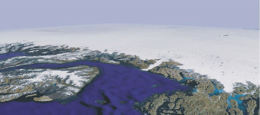
Disko Bay and Jakobshavn Isbræ, a calving outlet glacier from the Greenland Ice Sheet, seen from southwest. Jakobshavn Isfjord and Jakobshavn Isbræ is seen near the centre of the picture. Disko Island is seen to the left, and part of the Greenland Ice Sheet is seen in the background. The distance from southernmost Disko Island to the mouth of the ice-filled Jakobshavn Isfjord (Ilulissat Icefjord) is about 100 km. Picture source: Google Earth.
The Disko Bay region in central West Greenland (c. 70oN) is characterised by large outlet glaciers from the Greenland Ice Sheet (the Indland Ice). The major glacier Jakobshavn Isbræ is situated in a major subglacial valley, which can be traced inland for about 100 km (Echelmeyer et al. 1991). The water depth in the fjord reaches 1500 m in its outer parts (Iken et al. 1993).
The first thorough glaciological studies in this area were those by Rink (1853), who introduced the terms Inland Ice and ice streams. The Disko Bay was deglaciated rapidly around 10.500-10.000 years ago, in the early part of the present interglacial (Weidick 1968). When the retreating ice front reached the coastline at the mouth of the Jakobshavn Isfjord (Ilulissat Icefjord), the retreat was interrupted while the glacier front was resting on a bank near Ilulissat 200-300 m below the present sea level. Later, the glacier again retreated, and reached the modern position c. 7.000 years ago. The retreat, however, continued, and by 5.000 years before now the glacier front was east of the modern position, about 20 km east of the ice margin position in 1964 (Weidick et al. 1990).
Global cooling after 5.000 year before now resulted in significant growth of the Greenland Ice Sheet, and the resulting advance of Jakobshavn Isbræ culminated around the year 1850, during the Little Ice Age (se frontal position in the figure below). From 1851 the calving glacier began retreating, and at the end of the 19th century the glacier front was about 10 km east of the maximum position reached in 1851 (Bauer et al. 1968). The seasonal fluctuations of the glacier terminus were recorded 1879-1880 by Hammer (1883), who also described local inuit legends that the glacier-filled embayment Tissarissoq (see figure below) formerly was ice-free and used as a hunting locality. If this is correct, open water probably extented east of the early 21st century glacier front position before the onset of the Little Ice Age (Weidick et al. 2004).
Jakobshavn Isbræ is the main outlet glacier from the Greenland Ice Sheet, draining ice from about 6.5% of the total area of the ice sheet, and producing 30-45 km3 icebergs per year. This corresponds to more than 10% of the total output of icebergs from the Greenland Ice Sheet, and the Jakobshavn Isbræ is the most productive glacier in the northern hemisphere. The glacier flow velocity is also high, typically 20-22 meters per day. It is likely that the iceberg which sank Titanic in 1912 may have been produced by Jakobshavn Isbræ.
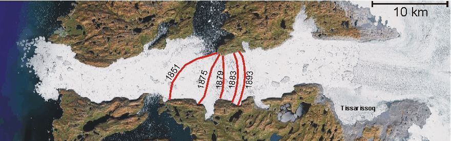
Frontal positions of calving Jakobshavn Isbræ in the latter half of the 19th century, after reaching the maximum Little Ice Age position around 1850 (Bauer et al. 1968). Between 1851 and 1893 the glacier front retreated about 10 km. The early 21st century (2001) glacier front is seen about 14 km east of the 1893 position. According to inuit legends, the embayment Tissarissoq used to be glacier-free and was used as hunting area (Hammer 1883), most likely before before the Little Ice Age glacier advance (Weidick et al. 2004). Picture source: Google Earth.
A note describing the retreat of Jakobshavn Isbræ 1893-1942 can be found here. A description of the glacier retreat in the early 21st century is found here.
Click here to jump back to the list of contents.
1854:
The Crimean War, beginning of systematic meteorological observations
The Crimean War (1853–1856) was fought between Imperial Russia on one side and an alliance of France, the United Kingdom, the Kingdom of Sardinia, and the Ottoman Empire on the other. The chain of events leading to Britain and France declaring war on Russia on 28 March 1854 can be traced to a fierce disagreement of whom was going to have "sovereign authority" in the Holy Land.
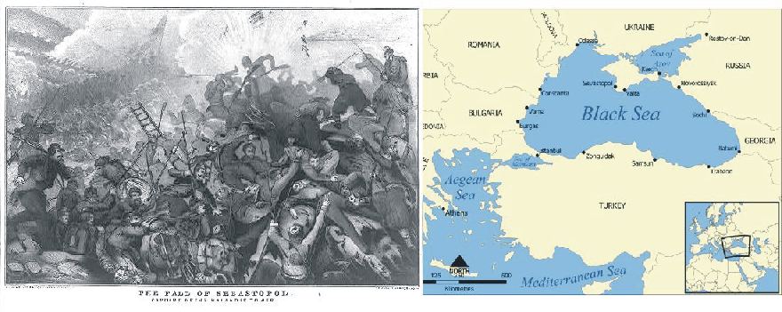
The fall of Sevastopol September 1855, after a year-long siege by the French and British fleets.
In
April 1854 allied troops landed in the Crimea and besieged the city of Sevastopol, home of the Tsar's fleet. During the siege, in November 1854, a
major part of the French-English fleet was destroyed in the
Click here to jump back to the list of contents.
1856-1857:
A severe winter in New England
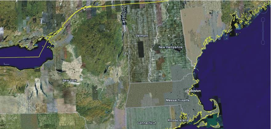
Northeastern USA with New England as seen in Google Earth.
The winter of 1856-57 was one of the severest winters ever known in New England, USA (Perley 2001). It began much earlier than usual, and continued far into the spring. There were 32 snow storms in total, three more than the average number for the preceding period, and the snow covered the landscape to a depth of six feet and two inches, while the 20 year average depth for eastern Massachusetts (Perley 2001).
The summer of 1856 had been hot, and the weather remained pleasant until mid December. On the night of 17 December extremely cold weather began. In both Massachusetts and Maine the temperature dropped to at least -12oF (-24oC), and the following day the temperature remained below 0 F all over New England, the coldest day recorded since 1836 (Perley 2001). On the night of 23 December there was a violent blizzard with much snow. Because of the high wind speed, several ships were lost along the coast.
On 3 January 1857 a new snow storm moved across New England, accompanied by a violent southeast wind. The railroads were more or less hindered by the snow which blocked their tracks. The air temperature was decreasing, and between 6 and 8 January became almost unbearable because of the wind and associated wind chill effects. Especially the western regions of New England suffered from snow and cold. In New Hampshire, on 12 January, the thermometer indicated -19oF (-28oC), and there was a very severe snow storm prevailing, accompanied by a gale that caused damage to the shipping along the coast. Provisions were sold at extremely high prices, and poor people suffered much for want of good and necessary food. Contributions for their benefit were taken in many of the churches in the cities (Perley 2001).
On the night of 17 January 1857, and also the next day, the cold was more intense than it had been during the previous part of the winter. At Salem, Massachusetts, the temperature was -20oF (-29oC). By evening the following day the temperature increased to 12oF (-11oC), but now snow began to fall. The wind was strong and from northeast. During the following night the wind increased until it became one of the severest and most violent that had been known for very many years. Snow fell to great depths, with drifts being 8 to 12 feet deep in Salem, Massachusetts. Also the streets in Boston were piled full of snow, and remained so three days later. Snow shoes were found to be necessary to pedestrianism, and many of the old ones were hunted up and brought into use again (Perley 2001).
The violent wind during this storm wrought many disasters on both land and sea. Buildings blew down, and the unusually strong wind over the ocean was very disastrous to the shipping. Many vessels were driven ashore and several lives were lost. At Provincetown, on northernmost Cape Cod, it was one of the worst storms ever experienced (Perley 2001). During and immediately following this storm, the temperature descended to an extremely low point, and remained there for a whole week. January 18 and 19 are supposed to have been the two coldest days known in New England during the 19th century (Perley 2001). At sunrise 19 January the mercury froze at Franconia, New Hampshire. At Montpelier and St. Johnsbury, Vermont, the air temperature was -50oF (-46oC), while it reached -52oF (-47oC) at Bath. The cold continued until 26 January. Long Island Sound became frozen for the whole width, and the harbour of Portsmouth in New Hampshire was frozen over as well.
This was one of the coldest winters ever known in USA, and it is said that the first snow storms known to have occurred in the city of Mexico was experienced this winter, on the night of January 31 (Perley 2001).
Click here to jump back to the list of contents.
1859:
John Tyndall conducts experiments on the radiative properties of various gasses
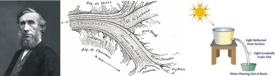
John Tyndall (left). John Tyndall's map of the French glacier Mer de Glace, where he in 1857 conducted glaciological investigations (centre). Experimental setup for one of John Tyndall's experiments (right), by which he, using a jet of water that flowed from one container to another and a beam of light, demonstrated that light used internal reflection to follow a specific path. As water poured out through the spout of the first container, Tyndall directed a beam of sunlight at the path of the water. The light, as seen by the audience in the lecture theatre, followed a zigzag path inside the curved path of the water. This simple experiment actually marked the first research into the guided transmission of light.
John Tyndall (1820-1893) was born in Leighlin Bridge, County Carlow, Ireland, the son of a part-time shoemaker and constable (Fleming 1998). At the age of eighteen, he joined the Irish Ordnance Survey as a draftsman and surveyor. During the period of railroad mania in UK, he worked 1844-1845 as a surveyor and engineer in Lancashire and Yorkshire.
In 1847, John Tyndall took a job teaching mathematics and drafting at Queenswood College in Hampshire, until he went on to study at the University of Marburg in Germany, where he completed a doctoral dissertation in mathematics. In 1852, Tyndall was elected a fellow of the Royal Academy, and one year later, with the support of Michael Faraday, he became a professor of natural philosophy at the Royal Institution of Great Britain. Here he focussed his research on the magnetic properties of crystals, the physics of ice, the transmission of heat through organic structures, and the radiative properties of gasses (Fleming 1998 and Wikipedia).
Starting in 1854, John Tyndall turned his attention to problems of geology and glaciers. This is not entirely surprising, as this was the time where the glacial hypothesis was getting its first foothold in mainstream scientific thinking, following the observations by Jean Agassiz in Scotland in 1840. He also developed an interest in meteorology, which at that time was beginning to receive widespread scientific interest as well, fuelled by the events during the Crimean War in 1854. Both of these interests presumably were also nourished by his keen interest in scientific mountaineering expeditions (Fleming 1998). He pioneered several solo attempts in the Alps, and climbed Mont Blanc (4807 m asl.) several times and was the first to climb the Weisshorn (4505 m asl.) in Switzerland.
In 1859, Tyndall begin a notable series of experiments on the radiative properties of various gasses. Inspired by his observations during mountaineering in the Alps, he established that the absorption of thermal radiation by water vapour and CO2 was of importance in explaining meteorological phenomena such as nighttime cooling, the formation of dew and frost, and possibly also changes of climates in the distant past (Fleming 1998). Tyndall's interest for past climate changes was clearly motivated by the contemporary debate of Agassiz's glacial hyphotesis.
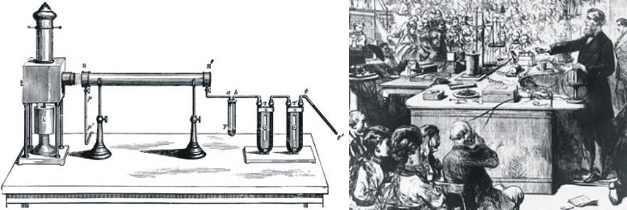
Experimental setup for one of John Tyndall's experiments, by which he investigated the infrared absorptive powers of different gases (left). John Tyndall lecturing at the Royal Society (right).
On May 26, 1859, John Tyndall announced some of his early results to the Royal Society, and two weeks later, he demonstrated his experiments to a distinguished audience at the Royal Institution. Tyndall's most striking discoveries were the significant differences in the abilities of different gasses to absorb and transmit radiant heat (Fleming 1998). During his different experiments, he measured the infrared absorptive powers of different gases, such as, nitrogen, oxygen, water vapour, carbon dioxide, ozone, and hydrocarbons. Based on this, he concluded that water vapour is the strongest absorber of radiant heat in the atmosphere and is the principal gas controlling the surface air temperature. Absorption by the other gases was found to be negligible. From these and other results, Tyndall pointed out that the role of water vapour "must form one of the chief foundation-stones of the science of meteorology." "It is perfectly certain that more than ten percent of terrestrial radiation from the soil of England is stopped within ten feet of the surface of the soil." "Remove for a single summer-night the aqueous vapour from the air which overspreads this country, and you would assuredly destroy every plant capable of being destroyed by a freezing temperature" (Fleming 1998).
According to Tyndall, water vapour "acts more energetically upon the terrestrial rays than upon the solar rays; hence, its tendency is to preserve to the earth a portion of heat which would otherwise be radiated into space." There could be no doubt about the "extraordinary opacity of this substance to the rays of obscure heat," particularly to the rays emitted by the Earth after its has been warmed by the Sun (Fleming 1998). Thus, Tyndall was the first to prove by experiments, what previously had been widely surmised by other scientists, that the Earth's atmosphere has a Greenhouse Effect (Wikipedia). Tyndall in his publications usually referred to radiant heat as "obscure radiation", "dark waves" or "ultra-red undulations", as the word "infrared" did not come into use until the 1880s.
John Tyndall attempted to link his laboratory results to meteorological experiments in the free air. For that reason he did some of his experiments on the roof of the Royal Institution in London. He quickly became worried about the disturbing influences of the city on his experiments, and was lead to consider London as a "heat island" and "a vast focus of artificial heat".
Earlier scientific contributions to the understanding of global climate dynamics can be found by clicking here and here. Later scientific contributions to the understanding of global climate dynamics can be found by clicking here, here and here.
Click here to jump back to the list of contents.
1872:
The Baltic Sea flood November 1872

Denmark and northern Germany seen from SW. Sweden and the Baltic is seen in the upper part of the picture. The different place names refer to localities affected by the 1872 Storm Surge, as outlined in the text below. The distance from Eckernförde to Bornholm is about 350 km. Picture source: Google Earth.
The
1872 Baltic Sea flood is often referred to as a storm flood. In the night of
12-13 November 1872 the storm ravaged the western Baltic
Sea coast from Denmark to Pomerania in northern Germany, and is considered
the worst storm surge ever recorded in the Baltic region in historical time. The
highest recorded peak water level was about 3-3.4 m above normal sea level
along the coasts affected, resulting in substantial flooding of adjoining land
areas and the loss of lives and property.
The 1872 storm surge took place in the final decades of the Little Ice Age (see diagram below), where storms in the North Atlantic were somewhat more frequent than now, mainly because of a somewhat larger thermal gradient between the Equator and the Arctic.
Anomalies
of global annual surface air temperature (MAAT) since 1850 according to Hadley
CRUT, a cooperative effort between the Hadley
Centre for Climate Prediction and Research and the University
of East Anglia's Climatic
Research Unit (CRU),
UK. The thin line represents the annual values, and the thick line is the simple
running 3 year average. The Baltic Sea Flood took place in a somewhat cooler
global climate than now.
In
the first week of November 1872 weather over northern Europe and the Baltic
region was calm (Hansen 1879, Petersen
1924). However, during November 7. the wind increased to storm from
directions initially SW and later NW over Denmark and northern Germany. The
strong NW wind resulted in water being driven into the western Baltic from the
North Sea and Kattegat between Denmark and Sweden.
Usually
there is a steady outflow of water (of relatively low salinity) from the Baltic
because of large rivers entering the Baltic, but now the situation for a couple
of days shifted to net inflow of water because of the strong NW winds. At the
town Sønderborg
at the Baltic coast in southern Jutland (Denmark) the sea water salinity by this
increased from 1.987% to 2.434% (Petersen 1924).
At the same time, the surface current in the sounds between the Danish islands
became southerly 6-8. November, instead of being northerly as is usually the
case (Colding 1981, Petersen
1924). Due to the net inflow the water level in the Western Baltic increased
to about 20-40 cm above normal.
Under normal conditions there is a surface gradient along the axis of the Baltic towards southern Denmark, to make the outflow of excess water possible, but now this gradient was suddenly reduced by the wind-induced net inflow of water, resulting in the accumulation of a huge water body in the eastern part of the Baltic (Colding 1981, Petersen 1924).
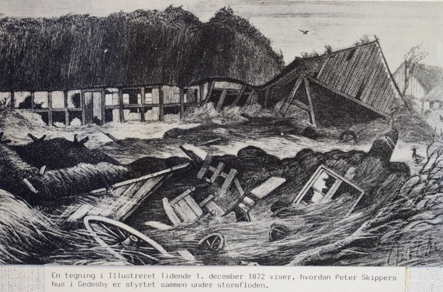
Drawing
in the Danish newspaper ‘Illustreret Tidene’ December 1, 1872. The
illustration shows a house belonging to Peter Skipper in Gedesby, southernmost
Falster, being destroyed by the flood and large waves during the Storm Surge in
the early morning of November 13, 1872. For location of Gedesby see
‘Climate4you update June 2013’. Picture source: Den
Gamle Købmandsgård, Gedser, 2013.
During
November 9 the wind began to reduce in force, and everything appeared to return
to normal, but then wind changed its direction. Initially this change was
recorded at the north coast of the German island Rügen. From morning November
10 the wind turned into NE, and began to increase in strength over the entire
western Baltic and later also the eastern parts. During November 11 the wind
increased to gale and then storm from NE on the next day. Later that day,
November 12, the wind increased to hurricane, to the knowledge of the author
until now the only recorded NE hurricane in this part of Europe. The area
exposed to the highest wind speed was the western part of the Baltic between Rügen
and the Danish island Bornholm south of Sweden.
By
this the water masses accumulated in the Baltic was forced towards the western
end of the Baltic, where the water level rapidly began to rise. Simultaneously,
the hurricane-force NE wind partly prohibited the natural drainage of the excess
water masses north into the Danish sounds (Petersen
1924).
In
the night between 12 and 13 November and during the following morning extensive
coastal areas along the western part of the Baltic was flooded by water masses
rising 3-3.4 m above normal. Huge waves caught coastal dwellers by surprise and
caused floods over a metre high in coastal towns and villages. Probably the NE
hurricane culminated in the early morning hours of November 13.
Many
of the flooded areas already had protective dikes before the storm surge, as
this was not the first severe flooding event to hit this part of northern
Europe, but almost without exception these dikes were no match for the storm
surge in November 1872.
Of
all the German coastal settlements, Eckernförde
(see map above) was most heavily damaged due to its location on the Bay of
Eckernförde which was wide open to the northeast, directly into the hurricane
wind. The entire town was flooded, 78 houses were destroyed, 138 damaged and 112
families became homeless. In Mecklenburg and West Pomerania 32 people lost their
lives on land due to the floods. In the Greifswald village of Wieck almost all
the buildings were destroyed and nine people drowned. Houses were destroyed as
far as the centre of Greifswald.
Peenemünde
was completely flooded.
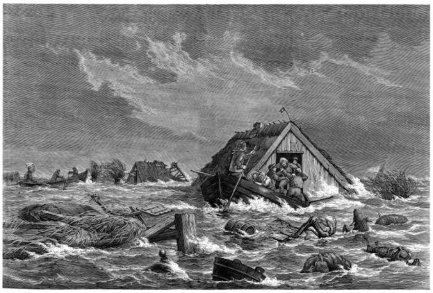
Contemporary illustration showing rescue efforts carried out in the early morning November 13, 1872, by people from the mainland of the Danish island Falster. Several houses from the village Bøtø near the eastern coast of the island were taken by the flood and drifted across the lagoon (Bøtø Nor) between the barrier island and the mainland to the west. The illustration shows a family being rescued from the still floating roof section of their house. Picture source: Det Lollandske Dige 2013.
The
Danish island of Lolland,
which has large areas protected by dikes, was badly hit and partly submerged and
28 persons lost their lives. On the Danish island Falster
farther to the east the situation was even worse, being exposed to the full
might of the NE hurricane. Dikes along the east coast of southern Falster were
rapidly overwhelmed and eroded away, and entire villages were destroyed by the
flood, resulting in the loss of 52 people. Many people scrambled to the top
floor of their houses as the water depth rapidly increased, but were trapped
inside without escape possibilities when the buildings subsequently collapsed
and were washed away by the waves (see drawing above).
In
total the flood cost the lives of at least 271 people along the Baltic Sea
coast; 2,850 houses were destroyed or at least badly damaged and 15,160 people
left homeless as a result. These numbers should be seen on the background of a
much smaller population than today. At sea about 260 ships were lost (Ejdorf
2003), amounting to the biggest shipping catastrophe in Denmark.
Statistically
the 1872 flood counts as a
100-year flood. A storm flood of similar dimensions today might cause far
more damage because the coastal region today is much more densely populated than
at that time. In many of the affected areas, however, dikes have now been
reconstructed with dimensions corresponding to the 1872 flood. Several places
these man-made dikes have later been reinforced by nature itself, as sand dunes
have been accumulating along the shore-side of them (see photo below).
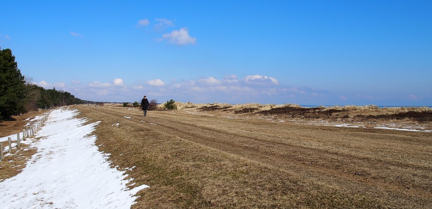
The
17 km dike along the southern part of the east coast of Falster was constructed
rapidly after the 1872 storm surge, and was finished in its present form already
in 1875. During the following 138+ years a ridge of sizeable sand dunes has
accumulated on the coastal side of the dike (to the east). The dike is seen in
the foreground, and the sand dunes to the right. View towards NNE. March 15,
2013.
Click here to jump back to the list of contents.
1874:
First Arctic meteorological stations established in Greenland

Mean annual air temperature at Godthåb (Nuuk) in West Greenland (64.2N, 51.8W). The thin line shows the annual values, while the thick line is the simple running 11 year average. Last year shown: 2007 (update 13 February 2009). Click here to download data since 1880.
The first systematic Arctic meteorological measurements are initiated in Greenland: Godthåb (Nuuk) in 1874, Upernavik in 1874, and Jakobshavn (Ilulissat) in 1874. The total mean annual air temperature record from Godthåb (Nuuk) is shown above, including a number of unofficial measurements from the time before 1874.
The main station in Godthåb (Nuuk) was established in 1872 (Brødsgaard 1992), but only from 1874 are official meteorological values published (see record below). The teacher Kleinschmidt, well known for his effort to establish a written version of the Greenlandic Inuit language, presumably was first to make meteorological observations in Godthåb in the years leading up to the opening of the official station.
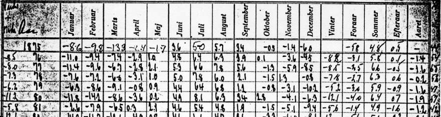
Part of the handwritten record with some of the first (1875) temperature observations from the meteorological station in Godthåb (Nuuk).
Click here to jump back to the list of contents.
1876:
The Merchant Shipping Act and the Plimsoll Sensation
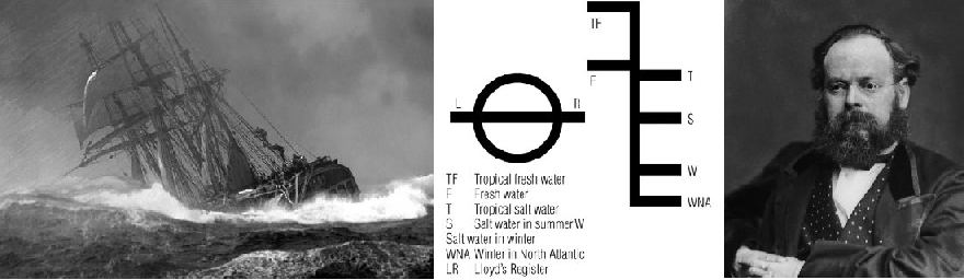
Ship in storm of the south coast of England around 1870 (left). The Plimsoll markings on ships; the long-awaited load line for different oceanographic conditions (centre). Samuel Plimsoll (right).
During the 19th century, British trade with the rest of the world was growing rapidly. The large number of ships being wrecked each year caused greater and greater concern. For example, in the year 1873-4, 411 ships sank around the British coast, with the loss of 506 lives. Between 1830 and 1900 about 70 percent of all sailing ships of the Tyne in England were lost a sea. During those same years one out of every five English mariners who embarked on a life at sea also died at sea (Jones 2006). Overloading and poor maintenance made some ships so dangerous that they became known as 'coffin ships', especially as gales and storms were frequent during the Little Ice Age.
By the 1870 Merchant Shipping Act in England sailors could be imprisoned for three months for breach of contract if they refused to board an unseaworthy ship once they had signed up for a voyage. Between 1870 and 1872, 1628 sailors were sent to jail in Great Britain for refusing to go to sea in ships they thought were unseaworthy.
In 1870, Samuel Plimsoll MP, who was a coal merchant, became interested in the subject. He began to write a book about the disastrous effects of overloading ships without respect to bad weather. When he began to investigate, Plimsoll found the problem was even worse than he had expected. He began to campaign in parliament with the aim of improving safety at sea. Many ordinary people became interested in his book and his campaign. In 1872, a Royal Commission on Un-seaworthy Ships was set up to look at evidence and recommend changes. Plimsoll was, however, defeated several times in parliament and ridiculed in public. Especially many ship owners were reluctant toward introducing regulations of ship loading.
Friday 10 February 1871 a storm blew up in the Channel and in the North Sea. Many ships went down because they were to heavy loaded to ride the waves, and many sailors lost their lives. There was a public outcry in Great Britain following this disaster. For Samuel Plimsoller (MP) this particular storm became the tipping point for public opinion.
On 12 August 1876, after years of negotiations in the English parliament a new Merchant Shipping Act was passed with the Lord's amendments (Jones 2006). The Art had 45 clauses. No 26 was ground-breaking: it made a load line on every ship compulsory. Thereby the storm of 10 February 1871 and the long work by Samuel Plimsoller established the famous symbol, of a circle, twelve inches in diameter, with a line through the middle, which popularly took Plimsoll's name.
The Merchant
Shipping Act of 1876 made load lines compulsory, but the position of the line in
the ship hull was not fixed by law until 1894. In 1906, foreign ships were also
required to carry a load line if they visited British ports. Since then, the
line has been known in the
Even in modern times, whenever controversies generating strong feelings arise, references are made and analogies drawn to the Plimsoll case.
Click here to jump back to the list of contents.
1879:
The Tay Rail Bridge
disaster in Scotland
A
deep depression with strong winds (Beaufort force 10-11) was passing across
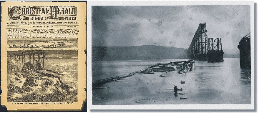
The Tai Rail Bridge disaster 28 December 1879, as documented by contemporary a contemporary newspaper. The old photograph to the right shows the central box-shaped section of the bridge lying on a sandbank in the river. The entire train, with the exception of the second-class carriage and the van, was contained within this section, explaining why nobody managed to escape drowning.
Today
there is still speculation as to the exact cause for the disaster, even though
the sheer force of the wind is seen as the fundamental cause (Burt
2004). One theory suggests that the bridge was not designed to withstand the
strong winds experienced in the evening of
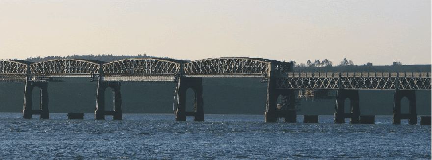
The new Tay Rail Bridge January 6th, 2008, looking SW. The old pier remains of the old bridge is seen below the modern bridge and provide a grim reminder of the 1879 disaster.
Click here to jump back to the list of contents.
1879-1881:
USS Jeannette sails for the North Pole
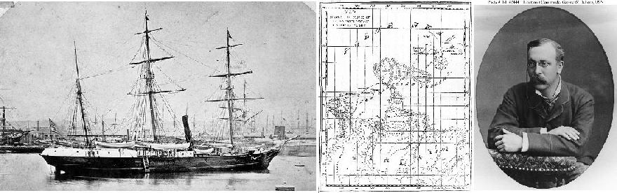
USS Jeannette (left).
Map showing the trek to the Siberian coast from the point
where USS Jeannette was crushed by ice (centre). Lieutenant
Commander George W. DeLong, USN
The
43 m long USS Jeannette was originally a gunboat (HMS Pandora) in the British
Royal Navy. In 1878 it was purchased by the owner of the New York Herald (James
Gordon Bennett, Jr.), and renamed Jeannette. Bennett was interested in the
The
Jeannette was modified and massively reinforced to allow her to navigate in the
Arctic pack ice. Lieutenant Commander George W. DeLong, USN, who had
considerable Arctic experience, was given the command. The crew consisted of 30
officers and men and 3 civilians. The ship contained the latest in scientific
equipment; and, in addition to reaching the Pole through
Bound
for the North Pole, Jeannette departed
On
The
two seperated parties began the long march inland over the swampy and half-frozen delta, hoping to find
settlements. One by one, however, members of DeLong's group died from starvation and exposure. Finally
DeLong sent his two strongest men ahead alone for help. They eventually managed
to find a settlement, but DeLong and the remaining men died before rescue arrived. The
other group under Melville was more lucky and relatively rapid found a native village on the other side of the
delta and were all rescued.
In
the summer of 1884 wreckage from the Jeannette was found on sea ice floes near
the southern end of
Click here to jump back to the list of contents.
1881:
Record number of polar bears arrive in Iceland
A record high number of polar bears arrived in Iceland during the winter 1880-1881 (Sturkell and Stockmann 2008). In total 63 bears made it to the shores of northern Iceland during the winter. Especially the coasts around the large embayment Húnaflói in northwestern Iceland has seen many visits of polar bears through time. In Iceland a young polar bear is referred to by the term 'Húna', and the occurrences of polar bears is seen in place names like Húnavatn (a lake) and the embayment Húnaflói. The community of Húnvatnsýsla represents another example, and carries very appropriately a polar bear in its official logo.
Click here to jump back to the list of contents.
1882:
First
IPY and early meteorological stations in the Russian Arctic

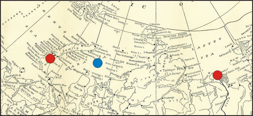
Part of map published by Taracouzio (1938), showing Soviet Arctic research stations in 1938. The position of the two Russian stations established during the First International Polar Year (IPY) is indicated by the red dots. The blue dot indicates the Kara Sea, where the ships transporting the Dutch and Danish IPY-expeditions got stuck in the sea ice in the late summer of 1882.
It
was in 1882 that the
first International Polar Year (IPY) was decided upon. It took
place from 1881 to 1884, and resulted in the first series of coordinated
international expeditions to the
Beginning
August 1882, various governments agreed to establish and maintain for at least
12 months a number of polar stations at various sites in the
Adverse
Little Ice Age sea ice conditions in the late summer 1882, however, blocked the Dutch
and Danish attempts of contributing to the first IPY. The ship “
Even
though both these attempts were unsuccessful in arriving at their planned
destination, the scientific observations made from both ships during the winter
1882-1883 proved of great value. In 1938 Taracouzio
stated that “even up to the present day the meteorological data on
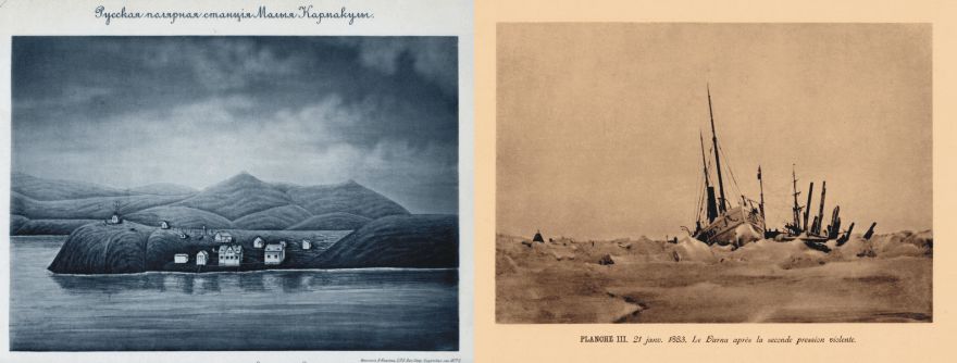
llustrations showing the Russian IPY station Malye Karmakuly on Novaia Zemlia (left), and the "Varna" caught in sea ice 21 January 1883 (right). Photo source: NASA information on the IPY history.
Click here to jump back to the list of contents.
1883:
The Krakatau volcanic eruption 
The explosive Krakatau eruption in Indonesia 27 May 1883 released huge amounts of ash into the atmosphere, giving rise to spectacular sunrise and sunset phenomena for a couple of years. Several painters have recorded this effect in their artwork.
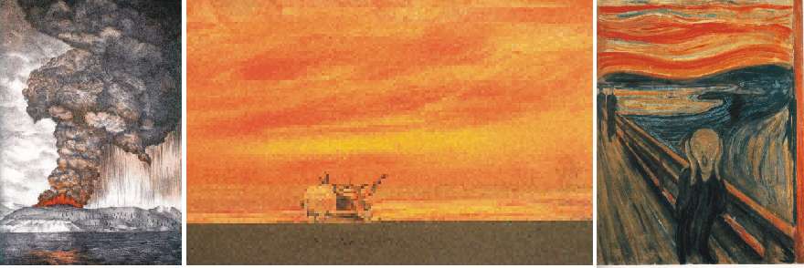
Painting of the Krakatau eruption 27 May 1883 (left). Oil painting 'Sunset' by Thames 23 Nobember 1883 (centre). The painting 'Skrik' (the Scream) 1893 by Edvard Munch (right). The dramatic skyline in this painting is thought to have been inspired by the global optical effects caused by the 1883 Krakatau eruption as seen over Oslofjord in the years thereafter.
Click here to jump back to the list of contents.
1884:
Glacier Vernagtferner in Austria begins to retreat from its Little Ice Age maximum
position
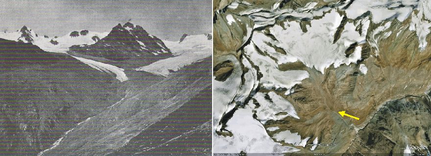
Vernagtferner (right) and Guslarferner (left) on 24 August 1884 (left part of illustration). Photo taken by Würthle and Son, from almost the same position as the 1844 water color by Thomas Ender, only a little higer up the valley side. Notice the clearly visible moraines on either side of the valley, above and in front of the glaciers. These moraines were formed during the 1844-48 advance. The right part of the illustration is an overview satellite picture showing Vernagtferner in 2007. The yellow arrow indicate the direction of view in the 1884 photo. Picture source: Google Earth.
Richter (1885) visited Vernagtferner in the summer of 1883, and used this occation to arrange for an early photograph of the glacier next year. This unique old photo was obtained on 24 August 1884 by Würthle and Son. Richter at the same time was seeking support for a precise mapping of the glacier from Deutscher and Österreicher Alpenverein. S. Finsterwalder directed the production of this very first photogrammetric map of the Vernagtferner in the years 1888 and 1889. This initiative resulted in continuous observation of the glacier ever since.
The 1844-48 advance of Vernagtferner was the last time that Vernagtferner reached and blocked the main valley Rofental. Since 1848 the glacier dynamics have been dominated by frontal retreat, interrupted by small readvances only. The present (early 21st century) retreat thus represents a continuation of a general development initiated around 160 years ago.
Click here, here, here and here to read about previous Little Ice Age advances of the Vernagtferner. Click here and here to read about the following glacier retreat during the warming period after the Little Ice Age.
Click here to jump back to the list of contents.
1895:
Arrhenius suggests that CO2 may trigger glacial advances and retreats

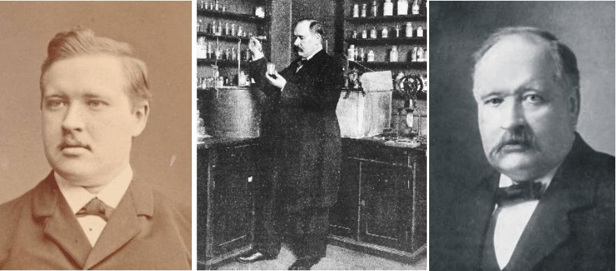
Svante August Arrhenius around 1884 (left). Svante Arrhenius in his laboratory in Stockholm (centre), and Professor Arrhenius around 1920 (right).
Svante August Arrhenius (1859-1927) is best known as an electrochemist who, along with Wilhelm Ostwald and Jacobus Henricus van't Hoff, pioneered the theory of electrolytic dissociation (Fleming 1998).
He was born in 1859 near Uppsala in Sweden. In 1876 he entered Uppsala University, where he followed a broad curriculum, including mathematics, physics, chemistry, Latin, history, geology and botany. In 1881, Arrhenius left Uppsala because of problems in the Physics Department, and instead went to Stockholm. There he came to work at the Institute of Physics of the Swedish Academy of Sciences with Erik edlund, a professor of physics who was interested in meteorology and who had ties to the Central Meteorological Office. Following the Crimean War (1853–1856) meteorology was becoming an issue of widespread scientific interest. In 1884 Arrhenius submitted his doctoral thesis on the chemical theory of electrolytes. The examination committee ignored certain theoretical aspects of this work, and did not award him the highest distinction. This was a severe blow to Arrhenius psyche and academic career, and he spend the next two years at home with his parents (Fleming 1998).
After a long postdoctoral period of six years and several unsuccessful candidacies, Arrhenius in 1891 obtained a lectureship in physics at the Stockholm Högskola (Stockholm College). In 1895 he became professor of physics at the same place. He was elected to the Swedish Academy in 1901, and his work on the electrolytic theory of dissociation earned him the Nobel Price for Chemistry in 1903. In late 1925 he suffered a stroke, and died in Stockholm after a brief illness on 2 October 1927.
Arrhenius was interested in general geophysics, although he did little experimental or observational work in geophysics. His basic approach was to apply physical and chemical principles to make sense of existing empirical observations. But as his grandson and biographer, Gustav O. S. Arrhenius, pointed out, "theoretical explanations of poorly known natural systems display a high mortality rate when confronted with accumulating evidence." Such was the general fate of Arrhenius's geophysical work, which served mainly as a catalyst for the more empirically based investigations of other scientists (Fleming 1998).
In 1895, while he was living home with his parents, he prepared a paper in which he suggested that a reduction or increase of about 40% in atmospheric CO2 might trigger feedback phenomena that could account for glacial advances and retreats during ice ages. As a result of Louis Agassiz's visit in Scotland, the glacial hypothesis had gradually gained support and general acceptance since 1850, which was the background for Arrhenius's interest in ice ages. The paper was presented to the Stockholm Physical Society, and published the following year (1896) under the title "On the Influence of Carbonic Acid in the Air upon the temperature of the Ground." In this paper he developed an energy budget for planet Earth, relying, among others, on the work of Josef Stefan's new law that radiant emission was proportional to the fourth power of temperature, and Samuel P. Langley's measurements of the transmission of heat radiation through the atmosphere.
Arrhenius in the 1895 paper made a number of very rough estimates of surface and cloud albedo and included simple radiative feedback effects in the presence of snow on the ground. At the same time, for simplicity, he ignored the effects of variations in horizontal heat transport and in the global cloud cover. Also the spectroscopic information available to Arrhenius was quite primitive. Arrhenius himself stated that for wavelengths greater than 9.5 microns, "we possess no direct observations on the emission or absorption of the two gasses (water vapour and CO2)".
Arrhenius argued that variations in trace components (including CO2) of the atmosphere could have a significant effect on the overall planetary heat budget. Using the best data available at that time, and making a number of simplifying assumptions (see above), he calculated the theoretical effect on the global temperature for a number of theoretical situations with reduction or increase in atmospheric CO2. Being primarily interested in the background for the onset of glaciations, he concluded that the temperature of the Arctic regions would rise about 8-9oC, if atmospheric CO2 increases to between 2.5 and 3 times its present value (Fleming 1998). Arrhenius understandably has a special interest in the modern Arctic regions, as he along with many contemporary scientists assumed that this was where future glaciations would initiate.
It is important to remember that Arrhenius was addressing the likely cause of the - at that time - newly accepted concept of "Ice Ages". From the onset, he showed little interest in the potential influence of human activity on the future chemical composition of the atmosphere. Instead, he wanted to evaluate the likelihood of great variations in atmospheric CO2 in relatively short geological times. For that reason he extensively referred to the research findings of his good friend and colleague, the Swedish geologist Arvid Gustav Högbom, who had worked on the geochemistry of carbon for several years. These geological research findings are described below. From Högbom's perspective, neither the combustion of fossil fuels nor the removal of organic carbon (deforestation) influenced atmospheric CO2 nearly as much as the different geological processes (Fleming 1998). Later, Arrhenius speculated about the potential warming effect of CO2 emitted by industry. On the time scale of hundreds to thousands of years, he thought that burning fossil fuels could help prevent a rapid return to the conditions of an ice age (Fleming 1998).
Earlier scientific contributions to the understanding of global climate dynamics can be found by clicking here, here and here. Later scientific contributions to the understanding of global climate dynamics can be found by clicking here and here.
Click here to jump back to the list of contents.
1895:
Arvid Högbom's
geochemical investigations on atmospheric CO2
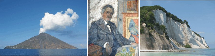
The volcano Stomboli, Italy (left). Swedish geologist Arvid Gustav Högbom (centre). Limestone rocks exposed on the island Møn, southeastern Denmark (right). These chalk formations were deposited in a tropical ocean covering Denmark about 65-70 mill. years ago, and were later pushed into their present, elevated position by the North European Ice Sheet, about 20,000 years ago, when Arctic climate conditions prevailed in most of Europe. By this, the above scenic Danish landscape is a geological visualisation on the existence of significant, natural global climate changes.
Simultaneously with the publication of Svante Arrhenius 1895 paper on the possible role for atmospheric CO2 as a control on glaciations, the Swedish geologist Arvid Gustav Högbom was working on the geochemistry of carbon. Arrhenius was using the findings of Högbom as an inspiration for describing a possible mechanism for variations in the amount of atmospheric CO2. Arrhenius and Högbom were both living in Stockholm; they were friends and colleagues, and of cause followed the research findings of each other with a keen interest. Following the acceptance of the glacial hypothesis after the observations of Louis Agassiz in Scotland in 1840, the mechanisms behind the onset of glaciations were becoming a scientific issue of widespread interest.
From Högbom's perspective, neither the use of fossil fuels nor the removal of organic carbon (deforestation) influenced atmospheric CO2 nearly as much as a suite of different geological processes. The formation of limestone and other carbonates was mentioned as one important mechanism, by which CO2 is removed from the atmosphere, and the decomposition of silicates, which adds to the atmospheric amount of CO2, was another mechanism. Also volcanic activity was emphasized by Högbom as an important agent adding CO2 to the atmosphere. Actually, Högbom considered volcanoes to be the "chief source of carbonic acid for the atmosphere" (Fleming 1998). In addition to this, he also mentioned the combustion of carbonaceous meteorites in the atmosphere as a possible, but virtually unknown, source for CO2.
Högbom estimated that the current atmospheric concentration of CO2 was of the same order of magnitude as the amount of carbon fixed in the living organic world. He further concluded that about 25,000 times as much carbonic acid is fixed in sedimentary formations in the form of limestone (see photo above) as is found in the atmosphere. On top of all this was the regulative role of the oceans, the potential importance of which was indicated by the research findings on the high solubility of CO2 in water by the English chemist William Henry as early as in 1803. As the carbon cycle thus contained several important processes, and because these in general could be considered independent of each other, Högbom stated that, from a geological point of view, a stable level of atmospheric CO2 was unlikely to persist at any time. In conclusion he therefore specified that the amount of atmospheric CO2 was likely to have varied considerably over time, as the result of different geological processes (Fleming 1998).
Having the assurance of Högbom that large variations in the atmospheric concentration of CO2 were quite likely in different geological periods, Svante Arrhenius in 1895 adopted this as foundation for his hypothesis explaining the onset of ice ages and interglacials as the possible result of natural variations of atmospheric CO2.
Earlier scientific contributions to the understanding of global climate dynamics can be found by clicking here, here, here and here. Later scientific contributions to the understanding of global climate dynamics can be found by clicking here.
Click here to jump back to the list of contents.
1897:
Chamberlin, geology, oceans and the carbon cycle 
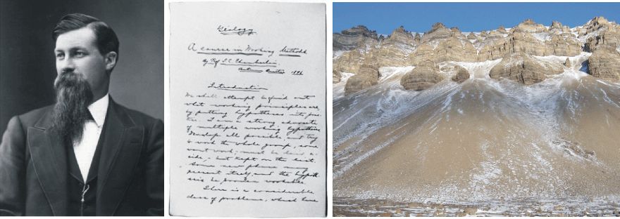
Thomas Chamberlin (left). One of Chamberlin's notes from his graduate geology seminar "A Course in Working Methods in Geology" at the University of Chicago (centre). Huge slopes (talus slopes) consisting of angular rock fragments derived from weathering line the foot of the mountain Templet (515 m asl.) on eastern Spitsbergen, Svalbard (right).
Thomas Chrowder Chamberlin (1843-1928) was born in a pioneer settlement near Mattoon, Illinois, USA. His father was a farmer and Methodist minister, and Thomas received a strongly religious upbringing. With time, however, Chamberlin would acquire equally strong geological interests, and eventually developed into one of the most outstanding American geologists ever. Chamberlin also made his mark in history by being the first of many geologists seeing the atmosphere as a fundamental geological agent.
In 1862, Chamberlin entered Beloit College. It was here he received his introduction to geology and scientific research from professor Henry Bradford Nason, an authority on chemical methods in geology (Fleming 1998). Because of Chamberlin's religious upbringing, he initially defended the geological doctrine of catastrophic deluges - the so-called Neptunist or diluvial theory. This hypothesis held that the record of geological rocks could be read in conformity with the biblical stories of creation and universal deluge. After studying the subject intensely and working with professor Nason, Chamberlin rejected this position as unscientific, and he decided to pursue a career as educator and geologist (Fleming 1998).
In 1869 Chamberlin obtained his first teaching position at the State Normal School at Whitewater, Wisconsin. In 1873 he joined the Wisconsin Geological Survey as assistant geologist, and serving as chief geologist from 1882. In 1881, Chamberlin also was appointed chief geologist of the Pleistocene division of the United States Geological Survey, a position he held for the next 23 years. By this, Chamberlin became an authority on glaciers, and was among the first geologists to identify a series of multiple glaciations in North America, in contrast to the previous belief in only one single glaciation. In 1887, Chamberlin became president of the University of Wisconsin, until he in 1892 moved to the new University of Chicago, where he was offered a position as professor of geology and chair of the geology department (Fleming 1998).
Each year at the University of Chicago, Chamberlin taught a graduate seminar in forefront geology research problems, entitled "A Course in Working Methods in Geology". One of the primary themes of the course was the geological significance of the atmosphere and its relationship to the great unsolved problems of the earth sciences, among them climatic variations leading to the recurrent glaciations, periods with extensive desert environments, as evidenced by salt and gypsum, periods with large accumulation of organic matter (coal deposits), and periods with decreases or increases in the number of species (Fleming 1998).
Inspired by the work of Tyndall and Arrhenius, Chamberlin in 1896 had the geological effect of atmospheric CO2 as overall course theme, and based on this, he in 1897 published a CO2 hypothesis of glaciation, entitled "A Group of Hypotheses Bearing on Climate Changes". Chamberlin proposed that variations of atmospheric CO2 combined with water vapour feedbacks could account for the advance and retreat of the past ice sheets. In this publication, although strongly inspired by the work of Arrhenius, he was critical of the idea proposed by Arrhenius and Högbom, that volcanism controlled the amount of atmospheric CO2. Instead, Chamberlin suggested that it was weathering of exposed bedrock which represented a main control on atmospheric CO2. In addition, he was the first to introduce the question of how much carbon was contained in various reservoirs, including the oceans, atmosphere, solid earth, and biosphere (Fleming 1998).
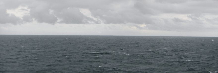
The North Sea east of Scotland on 29 September 2007. Oceans were pointed out as a large carbon reservoir by Thomas Chamberlin.
Chamberlin taught that over geologic time, the Earth had sequestered fantastic amounts of CO2 in various geological deposits. He estimated that the sedimentary rocks contained 16,000 times the amount of atmospheric CO2, coal beds 4,000, and oceans 18-22,000 times the amount of atmospheric CO2. In 1896 geologists knew that weathering of rocks dominantly consumes huge amounts of atmospheric CO2 and converts it to aqueous bicarbonates (e.g., Ca(HCO3)2), whereas the precipitation of calcium carbonates liberates CO2. From the work of William Henry it was also known that the amount of CO2 dissolved in the oceans would be inversely proportional to water temperature and salinity.
Based on this, Chamberlin formulated his carbon cycle dominated by geological processes. He saw chemical weathering of exposed rock as being a major factor for reducing the amount of CO2 in the atmosphere. Following periods with uplift of large land areas, or mountain building, the overall rate of weathering would be greater, and the atmospheric amount of CO2 smaller, than at times when low relief topography were dominating (Fleming 1998). The result of mountain building would then be global cooling, increased uptake of CO2 by the oceans, and possibly a glaciation. In case of glaciation, the extensive ice cover on land would hinder weathering and allow CO2 to increase in the atmosphere. Global warming would the be initiated with additional CO2 being released from the oceans, and additional warming assisted by water vapour feedbacks. After the glaciers had disappeared, large areas of eroded bedrock would be exposed for weathering (see photo above), whereby a new period of diminishing atmospheric CO2 and global cooling might be initiated. By proposing this hypothesis and also outline a global carbon cycle, Chamberlin was the first to argue in detail how geological processes might represent a dominant control on global climatic variations.
Chamberlin was convinced that variations in atmospheric CO2 and water vapour were significant for the global climate. Initially, he considered positive feedback mechanisms associated atmospheric water vapour to dominate. Later (1923), Chamberlin speculated on negative climate feedbacks, which he called "the adverse effect of H2O" (Fleming 1998).
In 1913, almost two decades after Chamberlin's initial work on the subject, however, the CO2 climate hypothesis had fallen out of favour. In a long letter to Charles Schuchert of Yale's Peabody Museum he wrote: "I have no doubt that you may be correct in thinking that the number who accepts the CO2 theory is less now than a few years ago... I greatly regret that I was among the early victims of Arrhenius error." The problem was that in 1900 Knut Ångström concluded that atmospheric CO2 and water vapour absorb infrared radiation in the same spectral regions, and that any additional CO2, it was argued, therefore would have little or no effect on the global temperature. In another letter written to Ellsworth Huntington in 1922, Chamberlin again expressed his deep regrets that he had overeagerly accepted Arrhenius's numerical results and that his "personal demon" had not kept Arrhenius's essay out of his way until after his 1897 paper had gone to press (Fleming 1998).
In 1922, towards the end of his commendable scientific career, Chamberlin thought that the role of CO2 in the atmosphere had been overemphasized and that not enough attention had been given to the role of the ocean, which he considered "my distinct contribution to the subject" (Fleming 1998).
Earlier scientific contributions to the understanding of global climate dynamics can be found by clicking here, here, here here and here.
Click here to jump back to the list of contents.
1899:
Thoughts about anthropogenic climate control
In 1899, the Swedish scientist Nils Eckholm, an early and eager spokesman for anthropogenic climatic control, pointed out that at present rates, the burning of coal eventually could double the concentration of atmospheric CO2. According to Nils Eckholm, being influenced by the thoughts of his lifelong friend and colleague Svante Arrhenius, this would "undoubtedly cause a very obvious rise of the mean temperature of the Earth." By controlling the production and consumption of CO2, he thought humans would be able to "regulate the future climate of the Earth and consequently prevent the arrival of a new ice age (Fleming 1998).
Eckholm, like his friend Arrhenius, thought warmer was better than cold. An increasing concentration of CO2 would counteract the expected deterioration of especially the northern and Arctic regions, as predicted by James Croll's astronomical theory of the ice age.
Click here to jump back to the list of contents.